monocle2
Monocle2 拟时序分析(未完成)
基本工作流
将数据储存在CellDataSet对象中
1 | pd <- new("AnnotatedDataFrame", data = sample_sheet)#储存对应seurat中的metadata信息 |
###对具有已知标记基因的细胞进行分类
根据已知的标记基因,对细胞进行挑选
1 | cth <- newCellTypeHierarchy() |
对细胞进行聚类
1 | cds <- clusterCells(cds) |
将细胞按照拟时间的轨迹进行排序
1 | disp_table <- dispersionTable(cds)#描述基因在每个细胞中如何随着平均值都变化而发生变化 |
开始Monocle的分析
- Monocle通常处理的是相对表达量,如:FPKM或者是TPM,或者是绝对的转录本计数,如:利用UMI试验方法还原出的数据
- Monocle也可以处理
CellRanger的转录本数据 - Monocle处理原始count数据时,可能会产生无意义的结果。在没有UMI计数结果的情况下,最好将原始数据进行标准化,使其成为TPM或者TPKM,而不是直接读入count。
CellDataSet的创建
Monocle包作用的对象是CellDataSet,这个类是BioconductorExpressionSet的派生。
创建CellDataSet,我们需要有三个输入。
| 变量 | 作用 |
|---|---|
| exprs | 一个数字矩阵,用于存储基因的表达量。行为基因,列为细胞。 |
| phenoData | 一个AnnotatedDataFrame对象,用于存放细胞样本的信息,类似于seurat中的meta.data,每一行是细胞样本,列是特征数据 |
| featureData | 一个AnnotatedDataFrame对象,用于存放feature信息,每一行是feature(如基因),列是基因的各种属性 |
对于输入文件的维度要求
对于表达矩阵:
- 具有与phenoData 具有的行数相同的列数,同时名称匹配
- 具有与 FeatureData 数据框架具有的行数相同的行数,同时名称匹配
注意:
- featureData的一列应该命名为:“gene_short_name”
通过以下代码可以创建:
1 | pd <- new("AnnotatedDataFrame", data = HSMM_sample_sheet) |
对于输入文件的标准化需求
- UMI数据:不需要在创建
CellDataSet前进行标准化,也不要将它转换为TPM或者FPKM
从其他包中导入或者输出数据
Monocle 能够将包“ Seurat”中的 Seurat 对象和包“ scater”中的 SCESets 转换为 Monocle 可以使用的 CellDataSet 对象。(本人试验导入失败)
1 | #导入seurat或者SCESet |
Monocle 也可以导出CDS到seurat或者SCESets
1 | lung_seurat <- exportCDS(lung, 'Seurat') |
为你的数据选择一种分布(必须)
1 | HSMM <- newCellDataSet(count_matrix, |
FPKM/TPM 值通常是对数正态分布的,而 UMI 或读取计数更好地用负二项式建模。要处理 count 数据,在 newCellDataSet 中指定负二项分布作为 ExpressionFamily 参数:
| Family function | Data type | Notes |
|---|---|---|
negbinomial.size() |
UMIs, Transcript counts from experiments with spike-ins or [relative2abs()](https://rdrr.io/bioc/monocle/man/relative2abs.html), raw read counts |
Negative binomial distribution with fixed variance (which is automatically calculated by Monocle). Recommended for most users. |
negbinomial() |
UMIs, Transcript counts from experiments with spike-ins or [relative2abs](https://rdrr.io/bioc/monocle/man/relative2abs.html), raw read counts |
比negbinomial.size()稍微地精确些,但是速度远远慢于,适用于小的数据量。 |
tobit() |
FPKM, TPM | Tobits 是截断的正态分布。使用 tobit ()将告诉 Monocle 在适当的地方对数据进行log转换。不要自行转换它。 |
gaussianff() |
log-transformed FPKM/TPMs, Ct values from single-cell qPCR | 已经转换为正态分布的数据使用,尽管 Monocle 的一些特性可能不能很好地工作。 |
使用正确的分布!
使用错误的分布,可能导致不好的结果。
FPKM/TPM数据可以使用relative2abs()转换为绝对数据,然后使用negobinomial.size(),通常会比使用tobit()函数得到更加理想的结果。
处理大数据集
使用稀疏矩阵加速
1 | HSMM <- newCellDataSet(as(umi_matrix, "sparseMatrix"), |
如果你有10X Genomics 数据并且正在使用 cellrangerRkit,你可以使用它来加载你的数据,然后像下面这样传递给 Monocle:
1 | cellranger_pipestance_path <- "/path/to/your/pipeline/output/directory" |
Monocle 的稀疏矩阵支持由 Matrix 软件包提供。不支持其他稀疏矩阵包,如 slamM 或 SparseM
将TPM/FPKM值转换成counts(可选)
1 | pd <- new("AnnotatedDataFrame", data = HSMM_sample_sheet) |
估计尺寸与分布
最后,我们还将调用两个函数来预先计算关于数据的一些信息。Size主要和表达量的scale有关,dispersion主要用于之后进行差异化分析。
estimateSizeFactors() and estimateDispersions()只对于前面使用了 negbinomial() or negbinomial.size() 的对象是需要执行的,而且有用。
过滤掉低质量的细胞
1 | HSMM <- detectGenes(HSMM, min_expr = 0.1) |
| gene_short_name | biotype | num_cells_expressed | use_for_ordering | |
|---|---|---|---|---|
| ENSG00000000003.10 | TSPAN6 | protein_coding | 184 | FALSE |
| ENSG00000000005.5 | TNMD | protein_coding | 0 | FALSE |
| ENSG00000000419.8 | DPM1 | protein_coding | 211 | FALSE |
| ENSG00000000457.8 | SCYL3 | protein_coding | 18 | FALSE |
| ENSG00000000460.12 | C1orf112 | protein_coding | 47 | TRUE |
| ENSG00000000938.8 | FGR | protein_coding | 0 | FALSE |
1 | HSMM <- detectGenes(HSMM, min_expr = 0.1)#探测基因表达量过低的细胞 |
为细胞进行分类和计数
根据细胞类型进行分类
1 | # 从HSMM数据集的元数据中提取基因"MYF5"对应的行索引 |
1 | HSMM <- classifyCells(HSMM, cth, 0.1) |
这里首先创建了一个叫做CellTypeHierarchy的对象,用于细胞分类。
使用addCellType为细胞添加分类的依据,这样子生成的CellTypeHierarchy对象可以用于这些实验中所有细胞的分类。
分类的结果储存在CellDataSet中的CellType列中。
ClassifyCells
| 参数 | 作用 |
|---|---|
| cds | 你想要分类的CDS对象 |
| cth | CellTypeHierarchy对象(分类的依据) |
| frequency_thresh | 如果至少这个百分比的细胞符合细胞类型标记标准,则将其全部估算为该类型。 |
| remove_ambig | 是否移除类型模糊的细胞 |
| remove_unknown | 是否移除未知细胞 |
不使用Marker基因对细胞进行聚类(可选)
Monocle 提供了一个算法,可以使用它来计算“未知”细胞的类型:
该算法在函数 cluster Cell 中实现,根据全局表达式配置文件将单元分组在一起。
这样,如果你的细胞表达了许多成肌细胞特有的基因,但恰好缺少 MYF5,仍然可以将其识别为成肌细胞。
clustercells 可以以无监督的方式使用,也可以以“半监督”模式,它允许用一些专业知识来帮助算法。
无监督模式
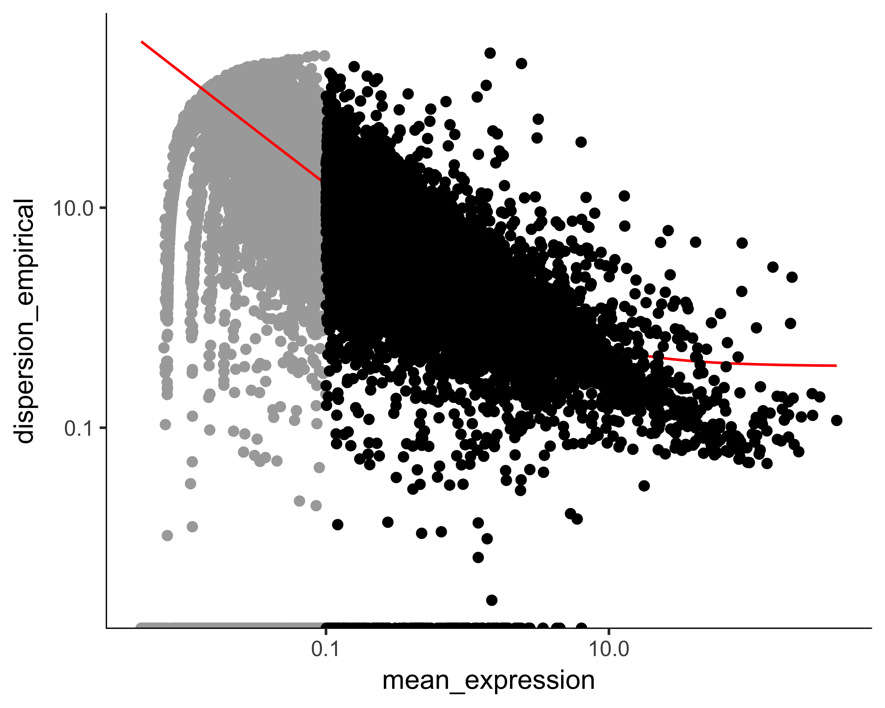
第一步是决定使用哪些基因来聚集细胞。我们可以使用所有的基因,但是我们会包括很多基因,它们的表达水平不足以提供有意义的信号。包括他们只会给系统增加噪音。我们可以根据平均表达水平筛选基因,我们还可以选择细胞间异常可变的基因。这些基因往往提供着关于细胞状态的大量信息。
1 | disp_table <- dispersionTable(HSMM) |
这里我们使用了自动筛选出的基因,用setOrderingFilter来对基因进行标记并聚类,此外,我们也可以自己指定基因进行筛选。
1 | HSMM <- reduceDimension(HSMM, max_components = 2, num_dim = 6, |
如果我们需要减去一些的无用的影响因素干扰我们的聚类,可以添加residuaModelFormularStr参数来减去指定的影响因素
1 | HSMM <- reduceDimension(HSMM, max_components = 2, num_dim = 2, |
使用Marker基因对细胞进行聚类
构建单细胞轨迹
排序工作流
Step.1 选择决定了细胞进展的基因
推断单细胞运动轨迹是一个机器学习问题。第一步是选择基因 Monocle 将使用作为其机器学习方法的输入。这就是所谓的特征选择,它对轨迹的形状有很大的影响。
Step.2 对数据进行降维
一旦我们选择了我们将用来排序细胞的基因,Monocle 就会对数据进行降维处理。
Monocle 使用反向图嵌入的算法来降维。
Step.3 将细胞按照拟时间进行排序
随着表达式数据投射到低维空间,Monocle 准备学习描述细胞如何从一种状态转变到另一种状态的轨迹。Monocle 假设轨迹有一个树状结构,一端是“根”,另一端是“叶子”。Monocle 的工作是尽可能地将最好的树与数据进行匹配。这项任务被称为流形学习一个细胞在生物学过程的开始,从根部开始,沿着树干发展,直到它到达第一个分支,如果有的话。然后,这个细胞必须选择一条路径,沿着树一直移动,直到到达一片叶子。
一个细胞的伪时间值是它返回根所需要的距离。
Step.1 选择决定了细胞进展的基因
Monocle中提供了四种方法:
- 选择发育差异表达基因
- 选择cluster差异表达基因
- 选择离散程度高的基因
- 自定义发育的marker基因
前面三种都是无监督的,最后一种是半监督。
选择clutser差异基因
1 | diff_test_res <- FindAllMarkers(seurat_object_name) |
使用Seurat选择高变基因
1 | ordering_genes <- VariableFeatures(seurat_object_name) |
使用Monocle选择高变基因
1 | diff_test_res <- dispersionTable(HSMM) |
使用发育差异表达基因
1 | #找到所有响应从生长培养基到分化培养基转变而差异表达的基因 |
Step.2 对数据进行降维
1 | HSMM_myo <- reduceDimension(HSMM_myo, max_components = 2, |
Step.3 将细胞按照拟时间进行排序
1 | HSMM_myo <- orderCells(HSMM_myo) |
此函数通常会出现问题,可以选择调用:
1 | # 6. 计算细胞拟时间 |
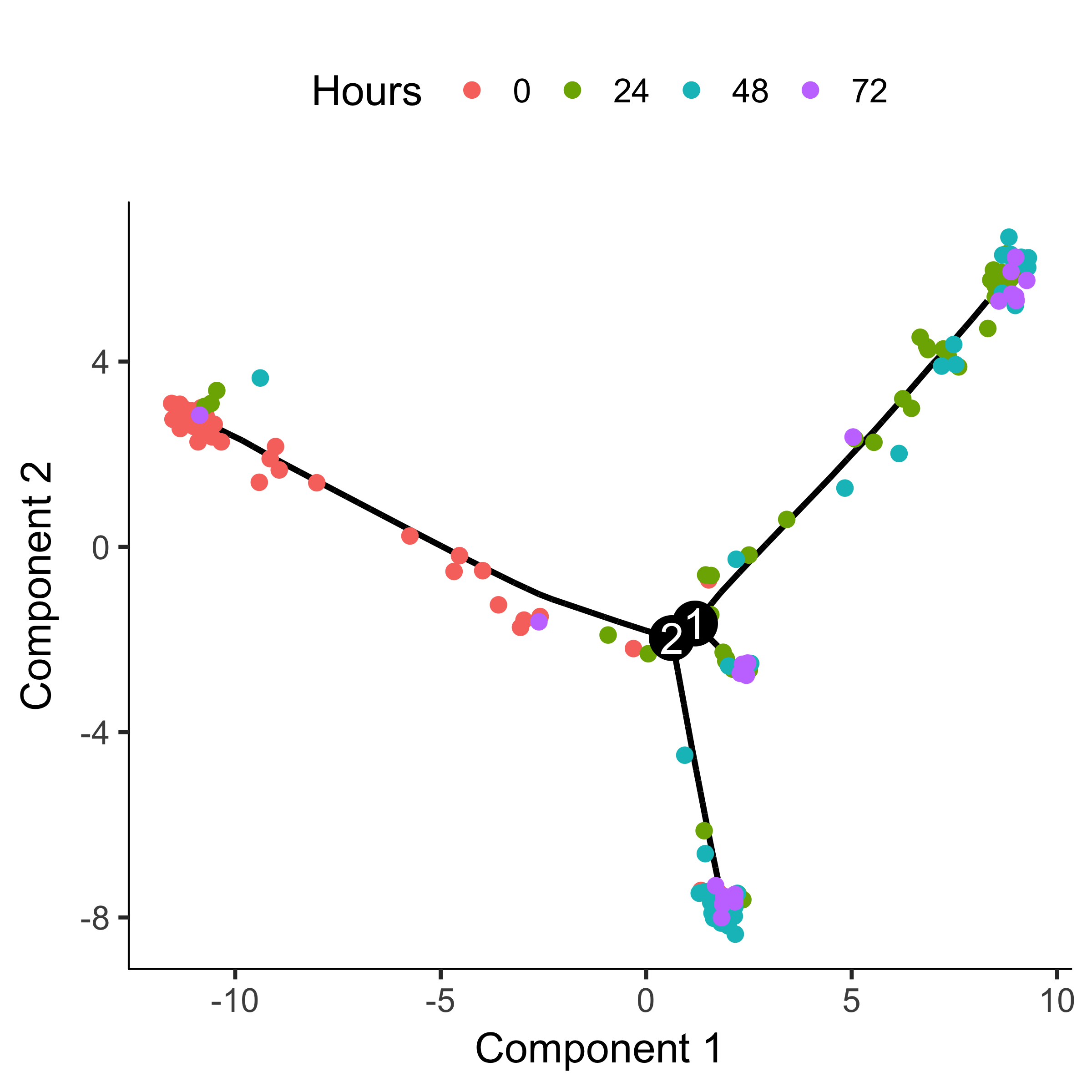
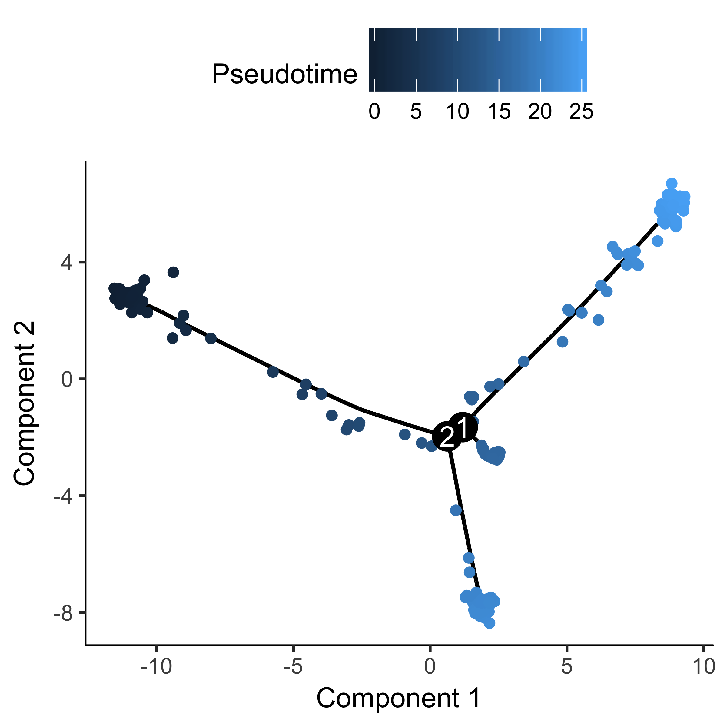
1 | plot_cell_trajectory(HSMM_myo, color_by = "Hours") |
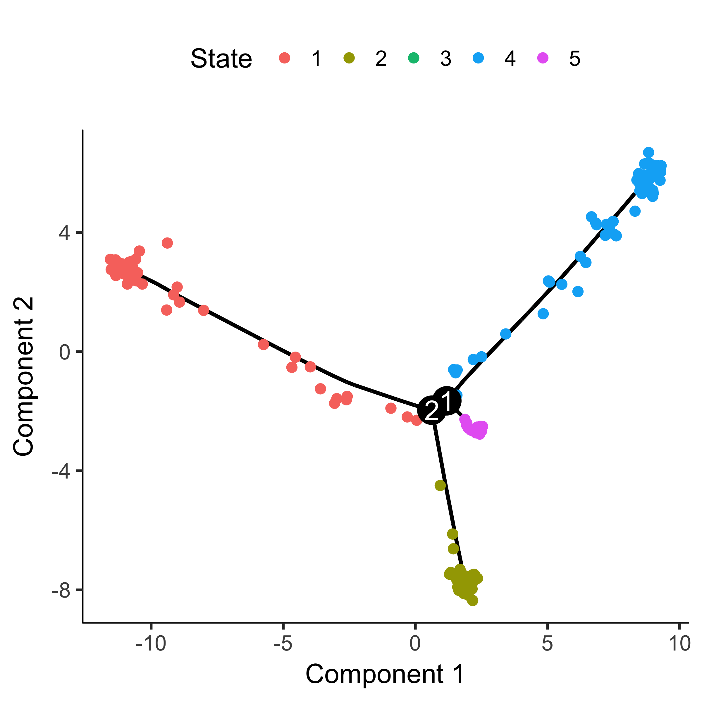
1 | plot_cell_trajectory(HSMM_myo, color_by = "State") |
1 | plot_cell_trajectory(HSMM_myo, color_by = "Pseudotime") |
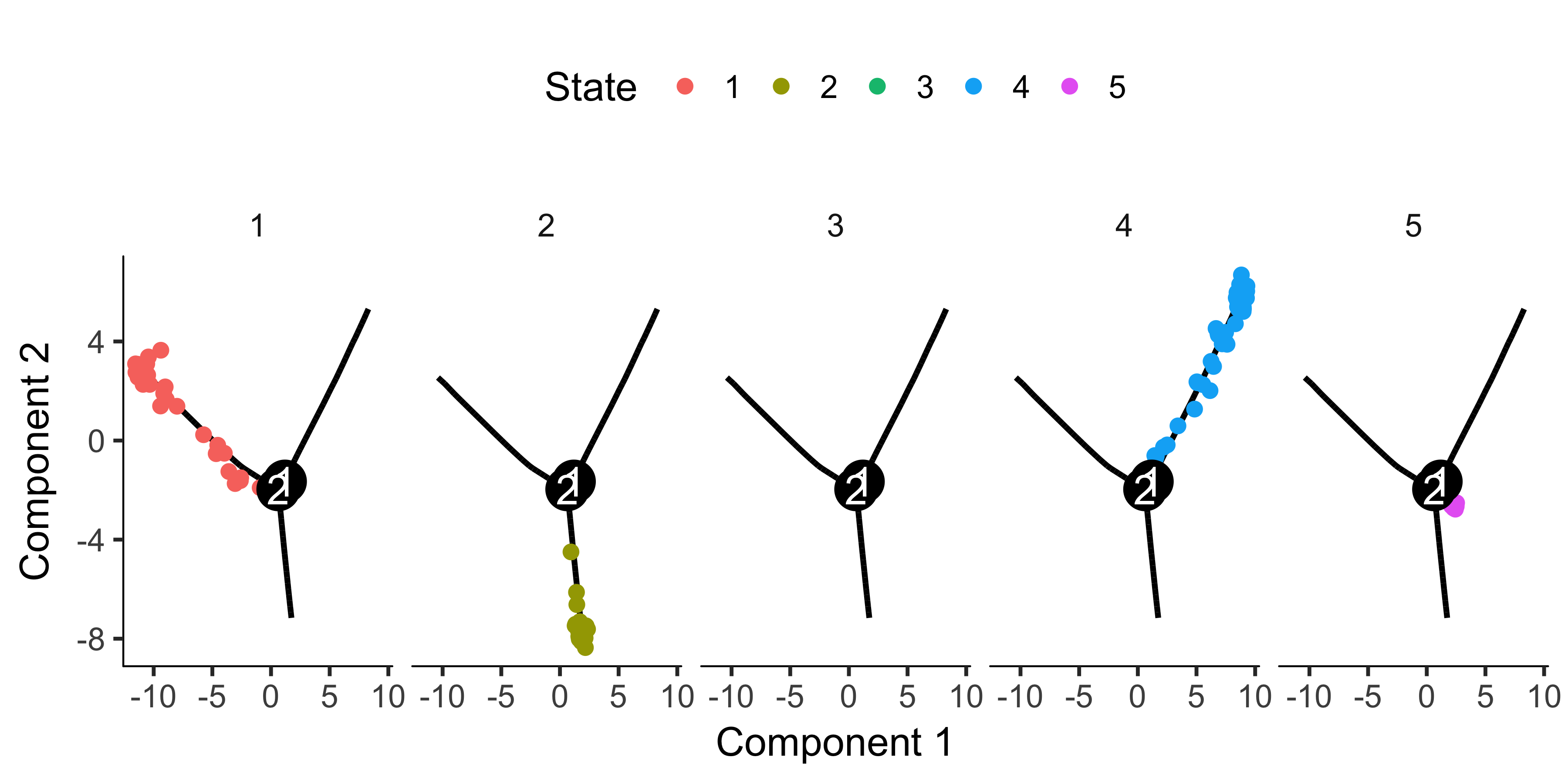
绘制分面的图
1 | plot_cell_trajectory(HSMM_myo, color_by = "State") + |
常用函数
| 函数 | 作用 |
|---|---|
| differentialGeneTest | 测试每个基因的差异表达,作为拟时间的函数或根据指定的其他协变量。differentialGeneTest是Monocle的主要差异分析程序。它接受一个CellDataSet和两个模型公式作为输入,它们指定由VGAM包实现的广义沿袭模型。 |
| detectGenes | 设置要与此CellDataSet一起使用的全局表达式检测阈值。统计CellDataSet对象中每个feature中可检测地表示为高于最小阈值的细胞数。此外,统计每个细胞中可检测到的高于该阈值的基因数量。 |
| setOrderingFilter | 该函数标记了随后调用clusterCells时用于聚类的基因。所选基因的列表可以在任何时候更改。 |